Running a Model and Viewing Results

Lesson 2, page 11 of 12

In order to simulate how a system A subunit of the world separated by a boundary from the rest of the world. The description of the system is comprised of the relations within the system as well as those characterizing the action of the outside world on the system. might evolve over time in a program like GoldSim, it is necessary to discretize time into intervals of time referred to as timesteps An element that generates discrete signals based on a specified rate of occurrence.. GoldSim then "runs the model" by "stepping through time", carrying out calculations every timestep, with the values at the current timestep often computed as a function of the values at the previous timestep.

Hence, in order to dynamically simulate a system in GoldSim, you must specify the duration of the simulation (e.g., 1 year) and the length of the timestep (e.g., 1 day). The appropriate timestep length is a function of how rapidly the system represented by your model is changing: the more rapidly it is changing, the shorter the timestep required to accurately model the system.

If you are running a probabilistic simulation A simulation in which the uncertainty in the input parameters is explicitly represented by defining them as probabilility distributions., you must also specify how many realizations of the model you would like to run. Recall from Lesson 1 that a realization A single model run within a Monte Carlo simulation. It represents one possible path the system could follow through time. represents a possible "future" for an uncertain system (i.e., one possible path the system may follow through time) and that running multiple realizations of a model is referred to as Monte Carlo simulation A method for propagating (translating) uncertainties in model inputs into uncertainties in model results..

After running a model, GoldSim can generate and display different types of results, in either graphical or tabular form. The two most common results viewed are the time history result A chart or table showing how a model variable changes with time. and the distribution result A chart showing the uncertainty in the output of a probabilistic simulation. Distribution results can take the form of a Cumulative Distribution Function, a Complementary Cumulative Distribution Function, or a Probability Density Function..

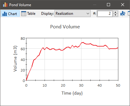
A time history result simply shows how a model output is predicted to change with time. As such, it is the fundamental type of result produced by a dynamic simulation model.The x-axis is time (or dates) and the y-axis is the value of the output. An example of a simple time history is shown below:

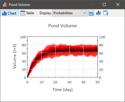
A probabilistic time history result (showing percentile bands) displays the range of outcomes that an output may have, accounting for the uncertainty in the model inputs.It looks like this:

A distribution result is the fundamental type of result produced by a probabilistic simulation. A distribution result shows a probability distribution A mathematical representation of the relative likelihood of a variable having certain specific values. of an output at a specific point in time (e.g., the end of the simulation):

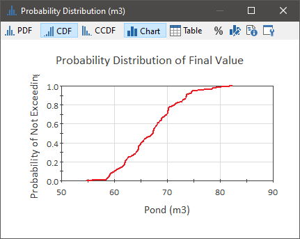
The particular type of chart shown above, referred to as a Cumulative Distribution Function (CDF) is the complement of the Complementary Cumulative Distribution Function A type of distribution result showing the uncertainty in the output of a probabilistic simulation. Typically referred to as the CDF. It is the integral of the probability density function. (CCDF) discussed previously in Lesson 1. The y-axis shows the probability of not exceeding the value on the x-axis.So in this example, if we look at an x-axis value of 60 m³, we see there is about a 10% chance that volume at the end of the simulation will not exceed that value (and hence a 90% chance that it will exceed that value).