Predicting Uncertain Outcomes Through Probabilistic Simulation
Lesson 1, page 3 of 5
The chart shown on the previous page could be the output of a single deterministic simulation. A deterministic simulation A simulation is which the input parameters are represented using single values (i.e., they are “determined” or assumed to be known with certainty). represents parameters, processes, and events using specified ("known") values, perhaps described as "the best guess", "typical", "best case" or "worst case" values. By running several deterministic simulations (e.g., best guess, optimistic inputs, pessimistic inputs) you could produce a qualitative statement such as this:
"If I don't change my spending habits, it is possible under some circumstances or scenarios that my account balance may go negative."
Such a statement is not particularly useful, however, since it does not discuss the actual likelihood of the account balance going negative.
In order to discuss actual likelihoods, it is necessary to be more quantitative about the uncertainty and variability in the parameters, processes and events controlling the system A subunit of the world separated by a boundary from the rest of the world. The description of the system is comprised of the relations within the system as well as those characterizing the action of the outside world on the system.. For example, in this case, it would be necessary to quantitatively describe the uncertainty in your spending habits.
Probabilistic simulation A simulation in which the uncertainty in the input parameters is explicitly represented by defining them as probabilility distributions. represents uncertainty explicitly and quantitatively. If an input is uncertain, it is defined using a probability distribution A mathematical representation of the relative likelihood of a variable having certain specific values.. If the inputs to a model are uncertain, the outputs are necessarily uncertain.Within GoldSim, the uncertainty in inputs is propagated to the uncertainty in the outputs using a technique known as Monte Carlo simulation A method for propagating (translating) uncertainties in model inputs into uncertainties in model results.. In Monte Carlo simulation, the entire system is simulated a large number (e.g., 1000) of times. Each of these simulations is referred to as a realization A single model run within a Monte Carlo simulation. It represents one possible path the system could follow through time. of the system, and represents a possible future (i.e., one possible path the system may follow through time). For each realization, all of the uncertain parameters are sampled (i.e., random values are selected from the specified distributions describing each parameter). Here is a time history chart showing 10 different realizations (10 equally likely possible futures) of the bank account value, explicitly accounting for uncertainty in the inputs:
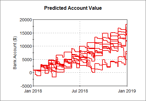
The 10 realizations are different due to the uncertainty in the input values (e.g., spending habits). The various realizations can subsequently be assembled into an output probability distribution (referred to as a distribution result A chart showing the uncertainty in the output of a probabilistic simulation. Distribution results can take the form of a Cumulative Distribution Function, a Complementary Cumulative Distribution Function, or a Probability Density Function.). This expresses the idea that if the inputs are uncertain, the outputs are uncertain.
The distribution result chart below shows the output of a probabilistic simulation of a large number of realizations (in which the uncertainty in spending habits is explicitly represented):
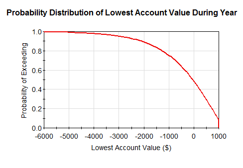
This chart displays the lowest account balance ever encountered during the simulation (i.e., over the entire year) as a probability distribution.This particular type of distribution result, referred to as a Complementary Cumulative Distribution Function A type of distribution result showing the uncertainty in the output of a probabilistic simulation. Typically referred to as the CDF. It is the integral of the probability density function. (CCDF) is quite simple to read.The y-axis shows the probability of exceeding the value on the x-axis.So in this case, if we go to $0, we see there is a 49% chance that the lowest account balance will exceed $0 (and hence a 51% chance it will become negative at some point). Hence, the result of a probabilistic simulation of a system is a quantified probability such as this:
"If I don't change my spending habits, there is a 51% chance that my account balance will go negative."
A quantitative statement such as this is much more useful than a simple qualitative statement.
Given such a result, you may choose to modify your spending habits (or find a better paying job)! To test this, you could assume some change (e.g., different spending habits, higher salary), rerun the model, and predict the likelihood that your account value will go negative.